

Understanding Differential Pulse Voltammetry
Applications in Biosensing

Differential pulse voltammetry (DPV) is a powerful technique for monitoring redox processes in electrochemical systems. It allows Faradaic currents to be resolved with high sensitivity against the capacitive background, enabling the detection of subtle electrochemical events that could be obscured in cyclic or linear sweep voltammetry.
However, DPV measurements are more complex and demand a more deliberate approach to experimental design. Unlike straightforward potential sweeps, the quality of a DPV signal depends heavily on parameters such as pulse amplitude, step potential, and pulse width, all of which directly influence sensitivity, resolution, and peak shape.
Unfortunately, people’s conceptual understating of what’s happening in a DPV measurement can be slightly off, making it difficult to to fully exploit the technique in the context of electrochemical biosensing.
In this article we will discuss:
How DPV measurements are performed and how the signal response is recorded.
Why DPV enhances Faradaic signals.
How pulse parameters (amplitude, width, step potential) influence peak shape, position, and sensitivity
Understanding DPV responses in the context of electrochemical biosensing
By the end, you should have a clear, intuitive understanding of what DPV is actually measuring, and how to tune it to extract reliable, high-quality data from real-world systems.
Differential Pulse Voltammetry
Unfortunately, some of potential vs time graphs describing DPV measurements in both research articles and text books can be slightly misleading. Typically, DPV is described as ‘‘a technique that involves applying amplitude potential pulses on a linear ramp potential.’’ You will commonly see graphical representations describing this:
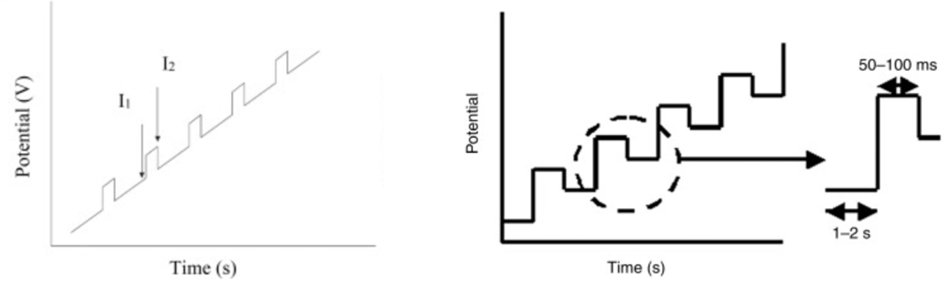
While these graphs (taken directly from ScienceDirect) illustrate the general principles of DPV, their representation can sometimes obscure which experimental parameters are actually critical for users to understand and control. This is especially true for researchers new to electrochemistry who may not have a full understanding of how potentials are applied, changed, and the resulting current recorded.
Let’s first create an accurate description of what is happening in a DPV measurement and then check to see if we think these graphs are accurately capturing what we are describing.
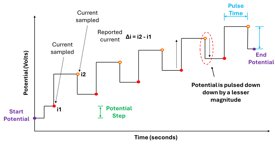
In DPV we are simultaneously sweeping the potential and applying potential pulses at discrete intervals. These pulses have a defined magnitude (pulse potential) and duration (pulse time), importantly the potential is constant over the duration of the pulse. The current is sampled (measured) just before each pulse is applied (i1) and just before the pulse ends (i2) , the current is then reported as the difference between i2 and i1 (figure 4).
Furthermore, in DPV when a potential is swept from some initial potential to some end potential this happens in discrete steps NOT as continuous linear ramp. The potential changes in steps: hold → jump → hold → jump (figure 2).
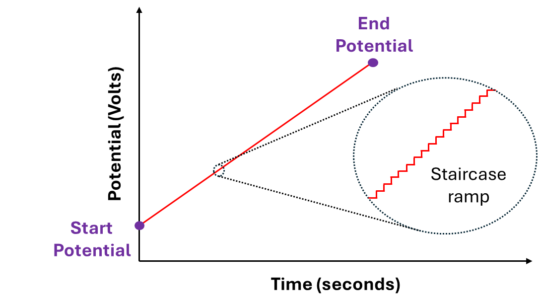
So now we have the added complexity of trying to conceptualise a potential being ramped up in discrete steps while we are also applying additional potential pulses along the way.
Furthermore, different potentiostat manufacturers describe the post-pulse transition differently: PalmSens treats the pulse as a temporary perturbation that returns to the step baseline, while Pine Research describes the potential as stepping back by less than the pulse amplitude, effectively combining the return and the next step into a single transition. Importantly, this has no effect on the measured current, as the DPV signal is determined solely by the current sampled immediately before the pulse (i1) and at the end of the pulse (i2), with all subsequent potential transitions occurring when the current is NOT being recorded.
Let’s summarise:
The potential is swept in discrete steps from some starting potential to some end potential.
Potential pulses are applied which have a defined magnitude and duration
The magnitude of the potential is constant for the duration of the pulse.
The current is sampled before the pulse is applied and before it returns to the baseline.
The current is reported as the difference between these two measurements.
It does not matter if the voltage returns to the same step potential before the pulse was applied or moves directly to the next step potential.
Let’s have a closer look at the graphs from figure 1 above:
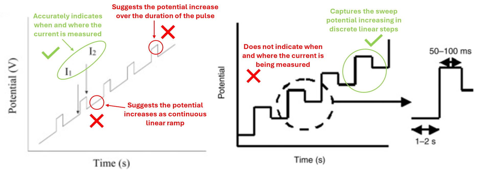
You can see from figure 3 above that the graph on the left is quite misleading and gives the wrong impression of how the potential is changing over time. The graph on the right is much more accurate and only omits when the current in being measured.
Lets create our own graphs to show in more detail what exactly is happening in a DPV measurement:
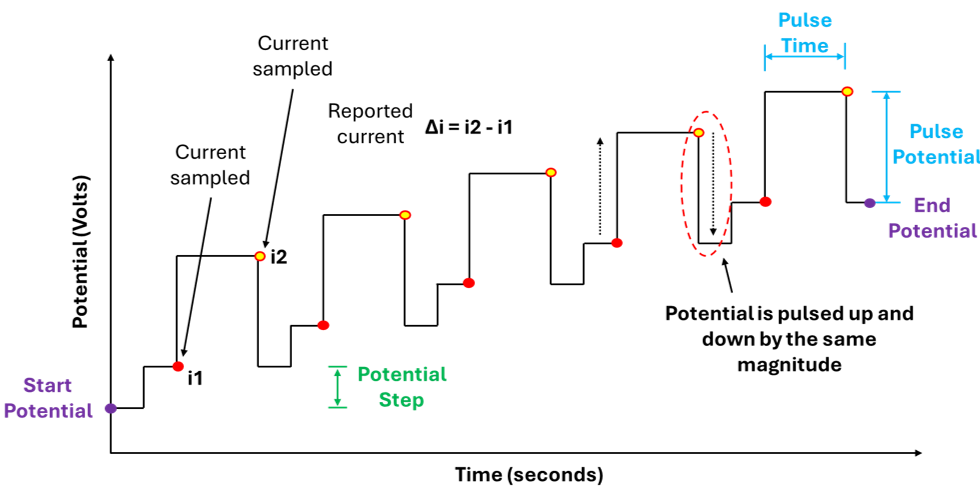
Both graphs in figure 4 above accurately capture our description of a DPV measurement, showing: The potential being increase via discrete steps (hold → jump → hold → jump), the potential pulses being applied along this potential pathway, the pulses themselves having a constant magnitude and duration, and when and where the current values are being measured.
Why Measure the Current like this?
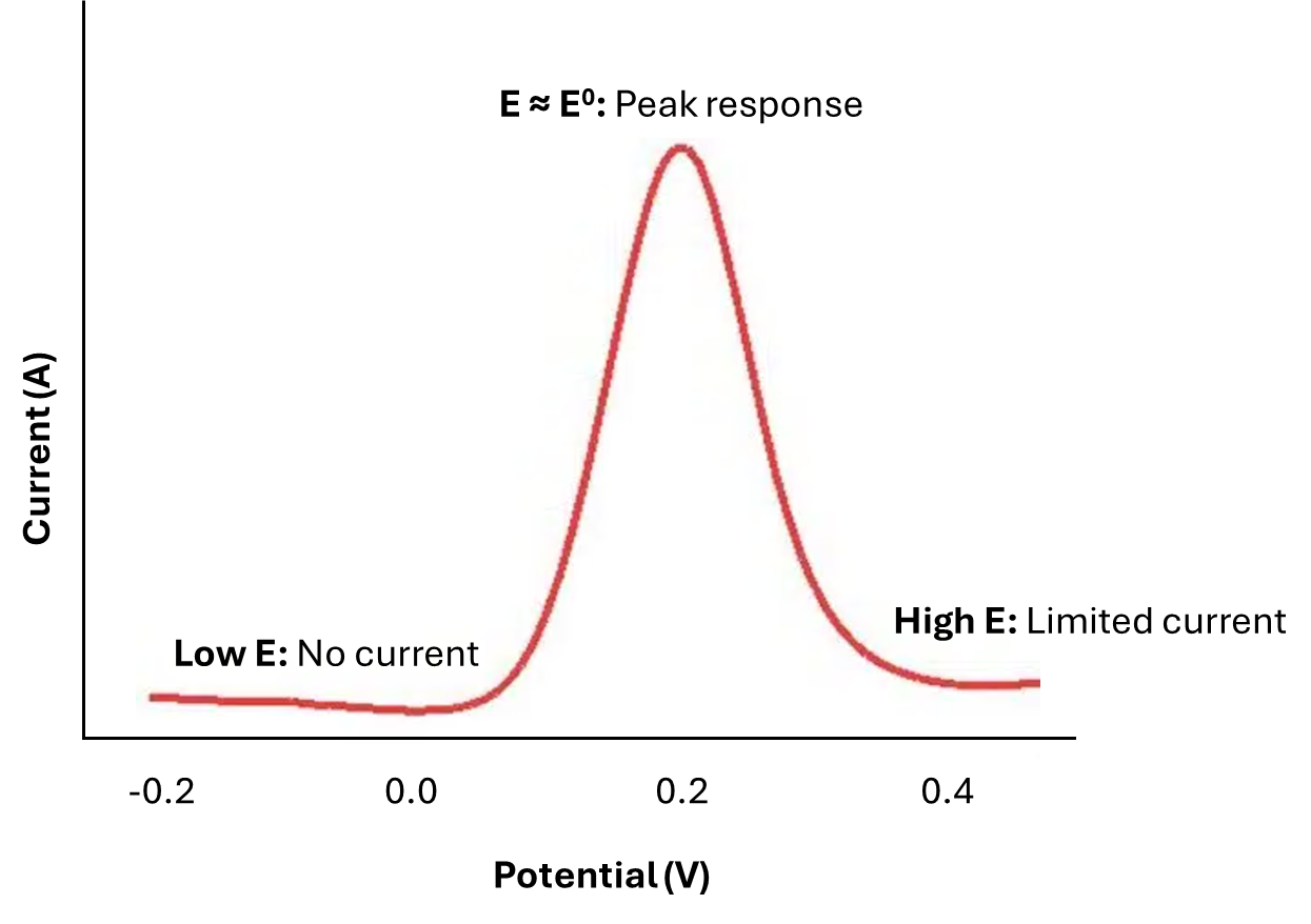
Let’s consider some species 'R' undergoing oxidation to 'O' at the electrode surface. The formal potential (E0) of the O/R couple is around 0.2 V, and we are going to sweep the potential from -0.2 to +0.5 V. Early in the experiment, when the applied potential is much more negative than E0, no faradaic current flows during the time before the pulse, and the change in potential during the pulse is too small to stimulate the faradaic process. Thus, the difference in i2-i1 (𝛿i) is essentially zero. Late in the experiment, when the applied potential is in the diffusion-limited region, 'R' is oxidised at the maximum possible rate. The pulse cannot increase the rate further; hence, the difference 𝛿i is again small. Only in the region of E0 (for this reversible system) is an appreciable difference in the faradaic current observed. There, the base potential is such that 'R' is oxidised at some rate less than the maximum, and the surface concentration of 'R' remains greater than zero. Application of the pulse forces 'R' to a lower value; hence, both the flux of 'R' to the surface and the faradaic current are enhanced, giving a significant 𝛿i. Only in potential regions where a small potential difference can make a sizable difference in current does the DPV show a response.
Setting Parameters in a DPV measurement
Below you can see a screenshot taken directly from PalmSens’ electrochemical analysis software (PSTrace - version 5.12) which shows the input parameters the user needs to set in order to carry out DPV measurements (at the moment the inputs are blank).
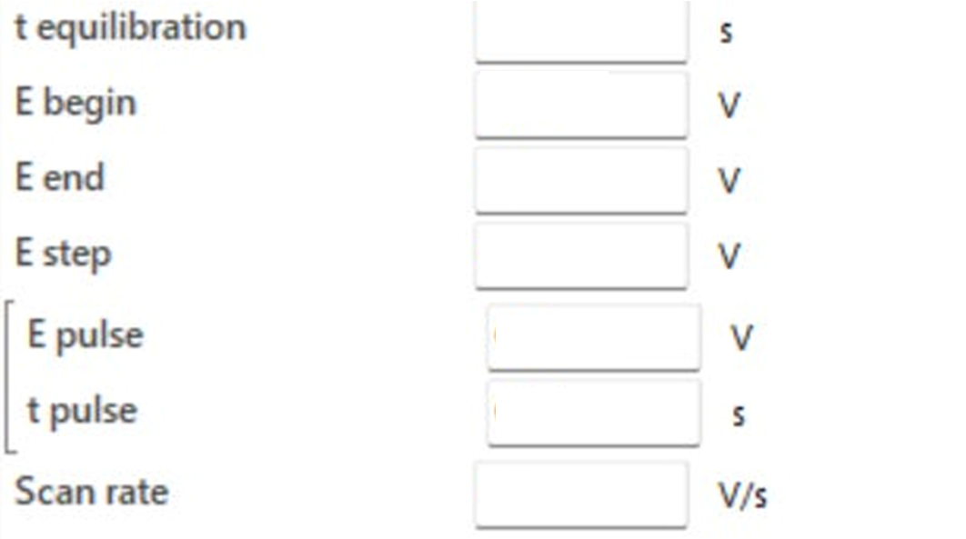
t equilibration (equilibration time)
This is the quiet time before the measurement starts. During this period, no potential scan is applied, allowing the electrochemical system to stabilize and the baseline current to settle before data acquisition begins.
E begin (starting potential)
This is the potential at which the DPV scan starts. It should be chosen so that it lies before the expected redox process of interest.
E end (end potential)
This is the potential at which the DPV scan finishes. It should be set beyond the expected oxidation or reduction peak so the full electrochemical response is captured.
E step (step potential)
This is the increment in base potential between successive measurement points. A smaller step potential gives higher resolution but increases the total measurement time.
E pulse (pulse potential)
This is the amplitude of the pulse superimposed on each potential step. It determines the size of the differential pulse used to probe the electrochemical response.
t pulse (pulse time)
This is the duration of each pulse. It affects both the measured current and the sensitivity of the method, since the current is sampled during the pulse.
Scan rate
This is the rate at which the potential is effectively swept during the experiment, usually expressed in V/s or mV/s. In DPV, it is determined by the relationship between the step potential and the timing parameters, rather than being an entirely independent setting.
Optimise what Matters
In electrochemical biosensing, not all parameters matter equally, some have a direct impact on sensitivity, resolution, and detection limits. Here’s how to think about the most important ones to tune and why they matter.
The pulse amplitude (E pulse) is a key parameter in DPV because it directly controls the magnitude of the differential current, which is measured as the difference between the current before and at the end of the pulse. Increasing the pulse amplitude enhances the perturbation of the redox process and therefore improves sensitivity, which is especially important in biosensing where signals are often small. However, excessively large amplitudes can distort peak shape and reduce resolution, so it is typically optimised by increasing it until a strong but well-defined peak is obtained, commonly within the range of ~25–100 mV.
The pulse time (t pulse) determines how long the system is held at the pulsed potential and influences how effectively non-faradaic (charging) current is suppressed. Since DPV samples current at the end of the pulse, the pulse duration must be sufficient to allow capacitive current to decay so that the measured signal is dominated by faradaic processes. In biosensing, t pulse is optimised by increasing it until baseline noise is minimised and the signal becomes stable and reproducible, while avoiding unnecessarily long experiment times; typical values are in the millisecond range.
The step potential (E step) defines the increment of the baseline potential between successive pulses and therefore determines the resolution of the voltammetric scan. Smaller step potentials provide more data points and better peak definition, which is crucial for resolving small or closely spaced signals in biosensing applications. However, smaller steps increase the duration of the experiment. In practice, E step is optimised by reducing it until no further improvement in peak clarity is observed, with typical values around 5–10 mV to balance resolution and measurement time.
DPV for Biosensing
A useful way to interpret DPV responses in electrochemical biosensing is to first ask what is actually being transduced at the electrode. In one class of assays, the redox-active species is surface-bound for example, a ferrocene, methylene blue, or enzyme cofactor tethered to a functionalisation layer. In the other class, the signal comes from a solution-phase species, either the target itself, a soluble mediator, or a product generated by an enzymatic reaction.
These two cases obey different physical limits, so the same “small peak” or “slow response” can mean very different things. In general, surface-bound systems are more often limited by electron transfer, molecular motion, binding kinetics, film transport, or probe crowding, whereas solution-based systems are more often limited by mass transport from bulk solution to the electrode and by depletion of analyte or mediator in the near-electrode region.