


From Theory to Practice: Leveraging Phase Shifts in EIS for Biosensors
Enhancing Biosensor Design Through Comprehensive EIS Interpretation

Electrochemical impedance spectroscopy (EIS) is a powerful analytical technique used to probe the dynamic processes occurring at the interface between an electrode and an electrolyte. It is widely utilised in the development and optimisation of electrochemical biosensors.
Many of you will be familiar with Bode and Nyquist plots and may have experience with modelling and/or extracting key parameters such as charge transfer resistance (Rct), double-layer capacitance (Cdl), and solution resistance (Cs). Typically, this information is extracted from EIS data plotted as frequency vs. magnitude or as the real vs. imaginary components of the impedimetric response. While these plots provide a wealth of information about the system’s electrochemical properties, one parameter that is often displayed by default in Bode plots but frequently overlooked or quickly removed is the phase angle.
In the biosensing literature, phase angles are typically only discussed when describing Nyquist plots – “diffusion processes lead to phase angles around 45° due to the Warburg impedance”, “a phase shift of 90° indicates ideal capacitive behaviour”, or “a 0° phase shift corresponds to purely resistive behaviour”. While these observations are valid, they only scratch the surface of what the phase angle can reveal about the system.
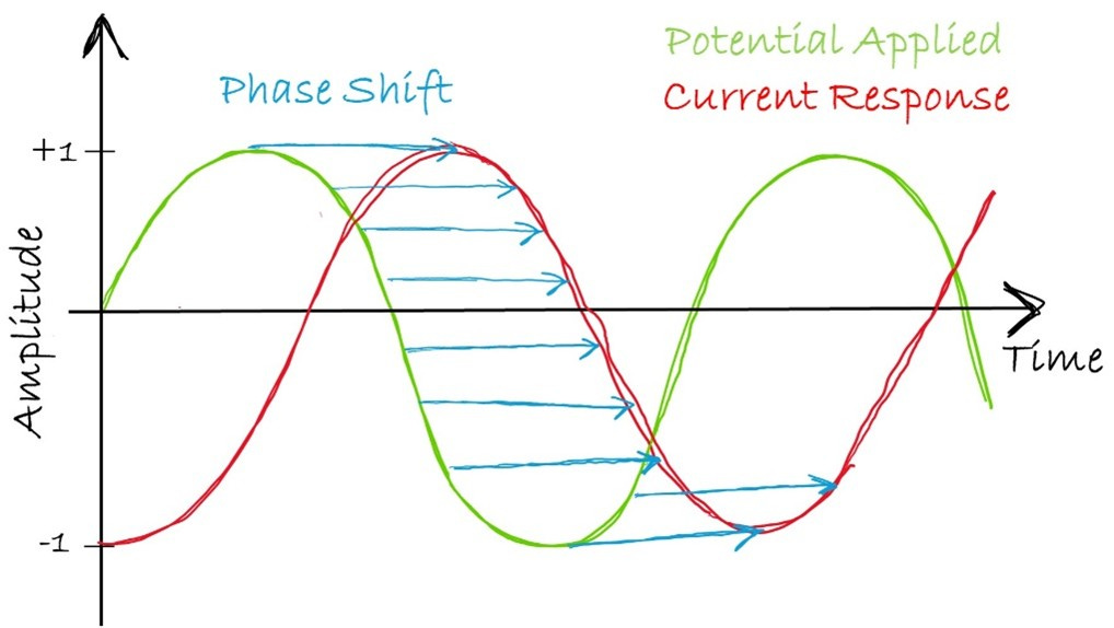
The phase angle in EIS originates from the inherent delay or shift between the applied alternating voltage (AC signal) and the resulting current response across an electrochemical system. This delay arises due to the presence of capacitive, resistive, and diffusional elements within the system (most common elements for biosensors), each of which affects the current response differently.
Let’s have a closer look at what’s going on.
When an AC voltage (typically sinusoidal) is applied to an electrochemical system, the resulting current does not respond instantaneously. Instead, it either lags or leads the applied voltage, depending on the nature of the system's components. This delay is quantified by the phase angle (ϕ), which is measured in degrees (°) or radians (rad).
In an ideal electronic circuit, the phase angle depends on the type of component:
Ideal resistor: ϕ = 0°
Ideal Capacitor: ϕ = 90°
Ideal Warburg diffusion ϕ = 45°
In the real world, ideal circuit components don't exist! The performance of components in your complex electrochemical system can deviate significantly from the idealised behaviour assumed in equivalent circuit models. When working with real electrochemical biosensors, it's crucial to consider:
1. The electrode surface is often rough, porous, or non-uniform due to fabrication defects, electrode wear, or intentional surface functionalisation.
2. Real-world components (acting as resistors and capacitors) are not ideal and have parasitic effects: These parasitic effects are frequency-dependent, meaning the impedance will deviate from ideal behaviour more prominently at high frequencies.
3. Real diffusion is rarely "perfect." Factors like restricted diffusion, boundary layer formation, or limited access to the electrode surface cause deviations.
It’s crucial to interpret the phase angle response in the context of your specific system, considering factors like the design of the sensing interface and whether a redox probe is being utilised. Without a redox probe, phase angle responses are mainly influenced by the intrinsic properties of the electrode, such as its capacitance and resistive contributions. While the presence of a redox probe can add complexity, it can also reveal deeper insights into electrode kinetics, surface modifications, and the performance of immobilised recognition elements.
Let’s have a look at how different circuit components affects the phase angle response across different frequencies:
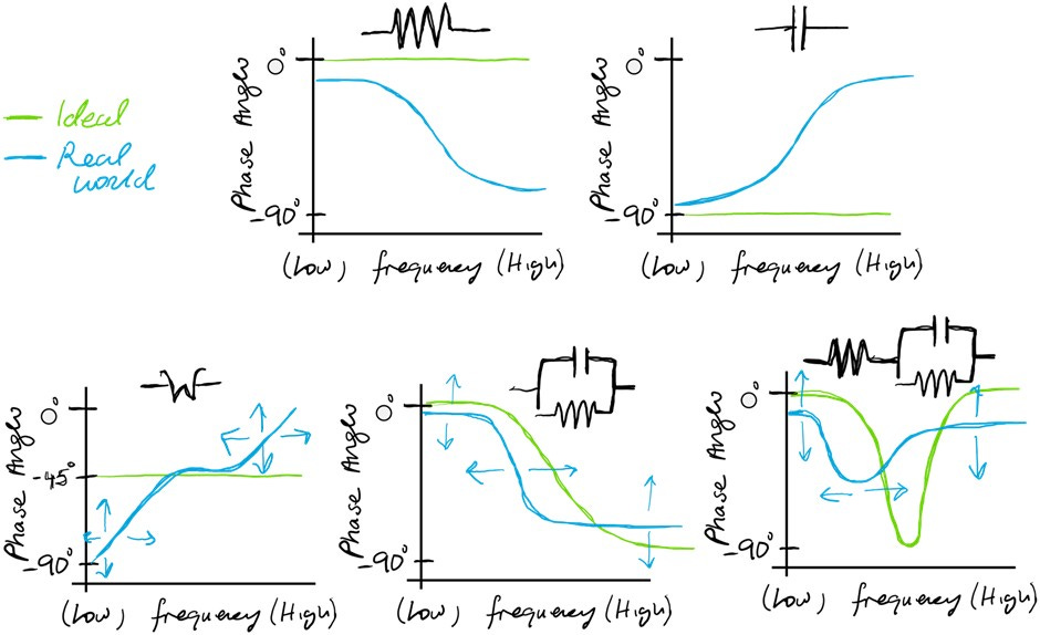
The blue arrows indicate how the response may vary in actual measurements of real systems.
Keep in mind that the responses illustrated above are only generalisations, real EIS measurements can vary significantly depending on many different factors. If you've designed your biosensing system from the ground up, you may be able to predict its phase response under ideal conditions. Comparing these predictions to the actual phase response can offer valuable insights into how your biosensor is performing and reveal limitations and/or deviations from the expected behaviour.
Moreover, the frequency-dependent nature of phase shifts opens the door to numerous practical applications, many of which remain underutilised in biosensor development:
1. Surface Modification
Surface modification is a crucial step in biosensor development, where the electrode surface is modified to immobilise biological recognition elements such as self-assembled monolayers (SAMs), antibodies, or aptamers. EIS can be used to confirm successful functionalisation by analysing the changes in phase shift.
Mechanism
Before functionalisation, the electrode typically exhibits a baseline impedance response, where the phase shift reflects the systems capacitance, charge transfer, and diffusion components.
After functionalisation, the immobilisation of molecules creates an additional dielectric layer on the electrode surface, this can increase the double-layer capacitance and modify the charge transfer resistance.
Bode Plot Observations
In a Bode plot, the increase in phase shift after functionalisation may appear as a shift in the peak phase angle to higher values at mid-range frequencies, confirming successful surface modification.
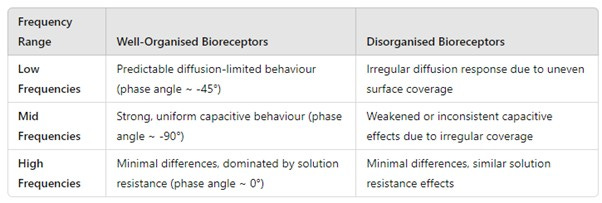
It may also be possible to determine how well organised your receptors are on the sensing interface:
2. Detection of Analyte Binding
One of the most critical applications of phase shift analysis is detecting biomolecular interactions, such as antigen-antibody binding, DNA hybridisation, or aptamer-analyte recognition. These binding events alter the interfacial properties of the biosensor surface, leading to measurable changes in the impedance response.
Mechanism
· When target biomolecules bind to immobilised receptors on the electrode surface, they can alter the local dielectric properties and the ability of charge to transfer across the interface.
· Binding events increase the double-layer capacitance and often increase the charge transfer resistance due to the insulating nature of biomolecules.
Bode Plot Observations
· Before binding: The Bode plot shows a moderate peak phase shift.
· After binding: The peak phase shift increases and may shift slightly in frequency depending on the extent of capacitance and resistance changes.
· Real-Time Monitoring: By continuously measuring the phase shift at a fixed frequency (e.g., 1 kHz), researchers can monitor binding events in real time, providing a label-free method for biosensing.
3. Rate-Limiting Step Identification
The phase shift can reveal the dominant process occurring in the biosensor, helping identify whether the system is limited by diffusion, charge transfer, or capacitance. The frequency range where the maximum phase shift occurs can indicate the rate-limiting step:
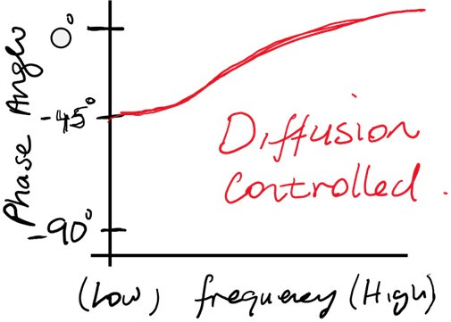
Diffusion Control
At low frequencies, the impedance is dominated by diffusion processes, described by the Warburg impedance.
Diffusion-limited systems exhibit a phase shift of approximately -45.
Example: The phase angle at low frequencies will stabilize near −45°, gradually increasing toward 0° as the frequency increases and diffusion effects diminish.

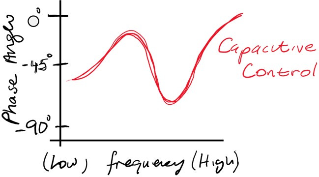
Capacitive Control
At mid frequencies, the impedance is dominated by the double-layer capacitance, especially after surface functionalisation or biomolecular binding.
The phase shift approaches -90° as capacitive behaviour dominates, reflecting the energy storage at the electrode-electrolyte interface.
Example: After immobilising a dense SAM layer, the phase shift at 1 kHz increases to 85°, indicating strong capacitive control.
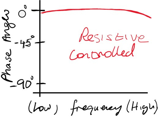
Resistive Control
· At low frequencies, the phase angle would remain close to 0° for a resistive-controlled system.
· At high frequencies, the phase angle still trends toward 0°, with small deviations due to parasitic effects.
· Example: At frequencies of 10 kHz or higher, the phase shift of a well-functionalised biosensor trends close to 0°, with small deviations reflecting the impact of parasitic effects in the system.
How to Analyse
By observing the phase shift across a wide frequency range:
If the phase shift is highest at low frequencies, the system is diffusion limited.
If the phase shift peaks at mid frequencies, the system is capacitive controlled.
If the phase shift is low across all frequencies, the system is resistive controlled.
Remember, for real systems, the phase response would unlikely be as clear as in the examples above. Typically, you would observe a mix of behaviours across different frequency ranges, with overlapping contributions from resistive, capacitive, and diffusive elements. However, understanding what to expect in terms of the phase angle if your system is controlled by resistance, capacitance or mass transport can help your better understand your biosensing system and carry out more targeted optimisations.
Comparing the phase angle response with other EIS parameters, such as charge transfer resistance (Rct), double-layer capacitance (Cdl), and Warburg impedance, can provide a more comprehensive understanding of the system’s behaviour. By correlating the phase angle data with these parameters, researchers can validate observations, identify inconsistencies, and gain greater confidence in the interpretation of their results. For instance, a phase angle indicating capacitive dominance should align with a low Rct and high Cdl, while deviations might suggest unexpected surface phenomena or fabrication defects. This multi-faceted approach ensures a more robust characterisation of biosensor performance.