


Affinity biosensors operate at the intersection of chemistry, physics, and engineering, relying on precise molecular interactions to detect specific analytes. Despite advances in sensor design, a fundamental bottleneck persists: accurately understanding and modelling binding kinetics. The interplay between association and dissociation events dictates the sensitivity, specificity, and real-world applicability of these sensors. This article explores the critical role of binding kinetics in biosensing, delves into the mathematical models used to describe these interactions, and highlights key challenges and opportunities.
1. The Fundamental Equations of Binding Kinetics
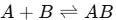
At its core, the interaction between an analyte (A) and an immobilised receptor (B) to form a complex (AB) can be represented as:
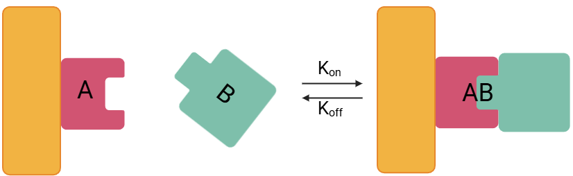
This reaction is governed by two key rate constants:
Association rate constant (Kon): The rate at which the analyte binds to the receptor.
Dissociation rate constant (Koff): The rate at which the analyte-receptor complex dissociates.
Mathematically, the rate of formation and dissociation of the complex can be written as:
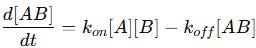
The first term (Kon[A][B]) represents the rate of complex formation.
The second term (Koff[AB]) represents the rate of dissociation.
At any moment in time, the net rate of complex formation depends on the balance between these two opposing processes. When the system reaches equilibrium, the rate of association is exactly equal to the rate of dissociation. This means the number of new complexes being formed is equal to the number of complexes breaking apart:
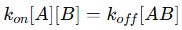
Rearranging this equation:
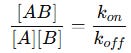
This ratio defines the equilibrium association constant (KA):
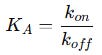
Alternatively, we define the equilibrium dissociation constant (KD), which is simply the inverse of KA:

KD represents the analyte concentration at which half of the receptors are occupied. If KD is low, it means the complex is very stable (low Koff ), so the analyte binds strongly to the receptor. If KD is high, it means the complex is unstable (high Koff), so the analyte does not bind strongly. In practical terms:
A strong binding interaction (e.g., antibody-antigen) has a low KD in the nanomolar (nM) or even picomolar (pM) range.
A weak binding interaction (e.g., transient protein-protein interactions) has a high KD in the micromolar (µM) or millimolar (mM) range.
Since biosensors rely on detecting biomolecular interactions, understanding KD is crucial for determining:
Sensitivity: A sensor must detect analytes at concentrations below or near KD for effective measurement.
Selectivity: If KD is too high, the sensor may detect non-specific interactions.
Real-time detection: Fast Kon and Koff rates allow rapid detection, while slow rates may lead to long response times.
This foundational equation underpins all binding kinetic models, from simple Langmuir adsorption to more complex stochastic and fractal-based approaches.
2. Mathematical Models of Binding Kinetics
While the simple Langmuir model works well under idealised conditions, real-world biosensing environments introduce complexity requiring more sophisticated models.
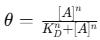
2.1. Langmuir Isotherm Model
The Langmuir adsorption model assumes a homogeneous distribution of binding sites and no interaction between bound analytes. The fractional occupancy (ϑ) , or the fraction of bound receptors, is given by:

where:
ϑ represents the proportion of occupied receptor sites,
[A] is the free analyte concentration,
KD is the dissociation constant.
This model is commonly used for kinetic fitting in surface plasmon resonance (SPR) and quartz crystal microbalance (QCM) experiments. However, it fails to account for surface heterogeneity and cooperative binding.
If you enjoy this content and would like to support it, please consider becoming a paid subscriber. For just £3.50/month get access to all Electrochemical Insights’ content .

2.2. Alternative Isotherm Models
Freundlich Isotherm
For heterogeneous binding sites with varying affinities, the Freundlich isotherm provides a more flexible approach:

where accounts for the heterogeneity of binding.
Fractal Kinetics Model
For heterogeneous surfaces, where binding sites have varying affinities, fractal-like kinetics describe the time-dependent decrease in reaction rates. The fractal kinetic equation modifies the standard Langmuir model:
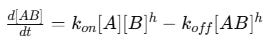
where h is the fractal dimension (0 < h < 1). This model accounts for molecular crowding and irregular surface topologies.
Cooperative Binding and the Hill Equation
In cases where multiple analytes bind to a receptor in a cooperative manner, the Hill equation is used:
where is the Hill coefficient, which quantifies the degree of cooperative binding.
2.3. Markov Chain Models
Binding kinetics can also be represented as a Markov process, where each molecular state transitions probabilistically to another. The transition probability matrix P defines the likelihood of moving from state i to state j in discrete time steps:
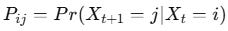
This framework is particularly useful for modelling stochastic binding events in noisy biological environments.
2.4. Langevin Equation and Brownian Motion
For diffusion-limited binding, where analytes must navigate through solution to find a receptor, the Langevin equation describes the motion of a molecule:
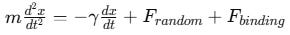
where ϒ represents viscous drag, and Frandom accounts for thermal fluctuations. This approach is critical for understanding biosensors operating in microfluidic environments.
2.5. Agent-Based Models (ABM)
ABM treats each analyte and receptor as an independent "agent" with defined rules for movement, binding, and unbinding. This method enables simulation of complex interactions, such as multi-valent binding and receptor clustering, which are difficult to capture with analytical equations.
3. The Challenges of Measuring Binding Kinetics
Complexity of Biological Samples: Clinical samples like blood, saliva, and urine aren’t pure solutions; they contain proteins, ions, and other molecules that can interfere with binding interactions. Nonspecific binding (NSB)—where unintended molecules stick to the sensor surface—can distort signals and lead to false positives or negatives.
Surface Chemistry and Receptor Orientation: Immobilising receptors onto a sensor surface isn’t as simple as just sticking them on. The way receptors are oriented affects binding efficiency. If they’re randomly distributed, only a fraction may be available for binding, reducing sensitivity.
Fouling and Secondary Interactions: In real-world applications, biosensor surfaces experience fouling, where biomolecules from the sample deposit onto the sensor, reducing performance over time. Secondary interactions, such as cooperative binding effects, can also alter expected binding kinetics.
Mismatch Between Lab and Real-World Conditions: Many binding kinetics studies are conducted under controlled conditions, but real-world applications require biosensors to function in unpredictable environments. Variations in pH, temperature, and ionic strength can all influence binding kinetics in ways that are difficult to predict.
Limitations in Measurement Techniques: Several technologies exist to measure binding kinetics, but each has its own strengths and weaknesses:
Surface Plasmon Resonance (SPR) – Label-free, high-throughput, but struggles with large molecules and NSB.
Quartz Crystal Microbalance (QCM-D) – Measures mass changes in real-time, but has lower sensitivity.
Isothermal Titration Calorimetry (ITC) – Provides thermodynamic insight, but requires high analyte concentrations.
Biolayer Interferometry (BLI) – Fluidic-free detection, but has challenges with low-affinity interactions.
Choosing the right technique depends on the application, but no single method provides a perfect solution.
4. Improving Electrochemical Biosensors with Binding Kinetics
Electrochemical biosensors offer a highly sensitive and cost-effective approach for detecting biomolecules, particularly in point-of-care applications. By integrating advanced binding kinetics models, we can enhance their performance in several ways:
Optimising Sensor Sensitivity
Electrochemical biosensors rely on detecting charge transfer events upon analyte binding. A well-characterised ensures that the sensor operates at an optimal analyte concentration range, maximising the response signal.
Reducing Nonspecific Binding and Background Noise
By incorporating models like Markov chains and fractal kinetics, we can better account for secondary interactions and surface heterogeneity, improving sensor specificity and reducing false signals.
Enhancing Response Times
Understanding the balance of and allows the design of biosensors that provide real-time measurements, crucial for medical diagnostics and environmental monitoring.
Accounting for Surface Modifications
Electrochemical sensors often require functionalised surfaces to immobilise receptors. Binding kinetics models help in predicting how modifications like self-assembled monolayers (SAMs) or nanostructured electrodes impact sensor performance.
Improving Stability in Complex Biological Matrices
In real-world applications, sensors encounter complex environments such as blood or wastewater. Advanced kinetic modelling allows us to predict and compensate for effects like biofouling and variable ionic strengths.
Multi-Valent and Cooperative Binding in Electrochemical Systems
Many electrochemical biosensors benefit from cooperative binding, where multiple recognition sites enhance the binding affinity and improve detection limits. Hill kinetics provides a useful tool for understanding and leveraging these effects.
By applying these kinetic models, electrochemical biosensors can be fine-tuned for enhanced performance, reliability, and broader applications in healthcare, environmental monitoring, and food safety.
Conclusion
Understanding binding kinetics is crucial for improving biosensor design. Whether through optimising analyte-receptor interactions, reducing noise, or enhancing sensor stability, the mathematical models explored in this article provide a roadmap for developing next-generation electrochemical biosensors with superior performance and real-world applicability.
Thank you for supporting Electrochemical Insights!

For a view of the history and critique of the Hill equation see “Hill in Hell” DOI 10.340277/Bindslev.208.14